The CAS Schedule P data is the Casualty Actuarial Society's free research database of loss triangles taken from US insurers' NAIC annual statements: six lines of business, ten accident years each with ten years of development, and, unusually, the later development as well as the triangle, so a method can be fitted on what was known at a year-end and scored on what happened next. That makes it the honest test bed for a reserve monitor. We replayed the comparison at the heart of Botminds' Loss Development Monitoring on it: freeze each insurer's triangle at the year-end, select a pattern, roll forward a year and flag any accident year that developed above its expected range. Across 1,700 accident years in the first data set, those flagged in the first year later proved adverse 51.7% of the time, against 20.7% for those not flagged.
Every number on this page from the replay is our own computation on the CAS's public files, with the method set out below so it can be repeated. It is not a result of the solution on any insurer's book; the screens show the solution's sample casualty book, with fictional companies and claims.
What a first-year flag said about an accident year's future, on two sets of closed data
52%
of accident years flagged in the first year later developed adversely (51.7%, 1997 freeze)
21%
of accident years not flagged later developed adversely (20.7%, 1997 freeze)
81%
of accident years flagged two years running later developed adversely (81.4%, 1997 freeze)
58%
flagged (57.5%) against 17.5% not flagged when the replay is repeated on the 2007 data set
What is the CAS loss reserving database?
The CAS loss reserving database is a set of six comma-separated files, one per line of business, posted by the Casualty Actuarial Society's research working group. Its stated purpose is narrow and useful: "The goal is to prepare a data set of loss triangles that could be used for claims reserving studies" (CAS). Each row is one insurer, one accident year and one development lag, with incurred losses, paid losses, bulk and IBNR reserves, and earned premium direct, ceded and net.
What sets it apart from simply downloading Schedule P is the squaring. The working group pulled each insurer's triangle from one year's annual statement and then filled in the lower half from the statements of the following years, so the outcome of every accident year is known to ten years of development. In the CAS's words, "Both upper and lower triangles are included so that one could use the data to develop a model and then test its performance retrospectively."
Where can I get Schedule P data, and which lines are in the CAS set?
The CAS files are free on the CAS research pages. Schedule P itself is part of the NAIC annual statement, and the CAS describes it as holding claims information on the major lines for every property and casualty insurer writing business in the United States (what each part of Schedule P holds is in Schedule P reconciliation); the CAS extract is the version a researcher can download, squared and cleaned. Two CAS sets exist: accident years 1988 to 1997, posted in 2011 as the set Meyers and Shi introduced, and accident years 1998 to 2007, which the CAS page marks as updated in December 2025.
The six lines are private passenger auto liability and medical, commercial auto and truck liability and medical, workers' compensation, medical malpractice on a claims-made basis, other liability on an occurrence basis and product liability on an occurrence basis. The variables come from four parts of Schedule P: incurred losses from Part 2, paid losses from Part 3, bulk and IBNR reserves from Part 4, and premiums from Part 1.
Are Schedule P triangles net of reinsurance?
Yes. The CAS page is explicit: "The triangles consist of losses net of reinsurance, and quite often insurer groups have mutual reinsurance arrangements between the companies within the group." For that reason the working group kept single entities, whether a whole group or a truly unaffiliated insurer, rather than every company in a group. Two consequences matter for a replay. A reinsurance program change moves a net triangle without any change in claims, and a monitor tested on net data is being tested on a harder problem than a gross monitor faces.
The losses also include defense and cost containment expense: the incurred variable is described as "Incurred losses and allocated expenses reported at year end", and the bulk variable covers IBNR on "net losses and defense and cost containment expenses". The reported losses in our replay, incurred minus bulk and IBNR, are therefore paid plus case reserves, including defense costs, which is the quantity a reserving actuary monitors.
How do you backtest a reserving method on Schedule P data?
You backtest by pretending to stand at an old year-end: use only the upper triangle known then, make the selections the method calls for, and score them against the lower triangle the method never saw. For a monitor the question is narrower than for a reserving model. Not "was the ultimate right?" but "when actual development broke above its expected range in the year after the review, did that accident year later prove adverse more often than the ones that stayed inside?"
How we replayed an actual-versus-expected monitor on the CAS Schedule P data
- Keep triangles a reserving actuary would monitor
Insurer-line triangles with at least $10 million of net earned premium over the ten accident years and positive reported losses in every known cell from the second lag: 284 triangles in the 1997 set, 321 in the 2007 set.
- Freeze at the last year-end
Use only cells known at 31 December 1997 (or 2007). Reported losses are incurred less bulk and IBNR, net, including defense and cost containment.
- Select a pattern and an ultimate
Volume-weighted chain ladder factors on all available years; the selected ultimate is the chain ladder projection. A real review selects with judgment; this is the mechanical stand-in.
- Draw an expected range at each age
The 10th to 90th percentile of the past age-to-age factors at that age, four to nine observations each: 80% of past variation, the solution’s default.
- Test the young accident years
Accident years at ages one to six at the freeze, where a range has at least four past factors behind it: six accident years per triangle.
- Flag in the first year after the freeze
When the actual factor is above the range and the unexpected, actual minus expected reported emergence, is more than 1% of the selected ultimate.
- Score against ten-year development
An accident year is adverse if its Schedule P incurred at the tenth lag, which includes the insurer’s own IBNR, is more than 5% above the ultimate selected at the freeze.
Two choices deserve a word. The 1% floor stands in for the solution's dollar threshold, which on a real book is set in dollars ($250,000 by default) so that small accident years do not flag on noise. And the 5% definition of adverse is deliberately modest; with a 10% definition the gap between flagged and unflagged years widens rather than narrows (on other liability frozen at 1997, 48.4% of flagged years against 17.4% of unflagged ones).
What the replay found: flagged vs later developed, line by line
On every line with enough insurers to read, accident years flagged in the first year after the review later developed adversely about twice as often as those that were not flagged, and those flagged two years running were adverse most of the time. The table gives the 1997 freeze by line and both freezes pooled.
CAS Schedule P data, replayed: flagged accident years later developed adversely about twice as often
| Line and freeze | Accident years tested | Later adverse, all | Flagged in year 1: later adverse | Not flagged: later adverse | Flagged two years running: later adverse | Adverse years the year-1 flag caught |
|---|---|---|---|---|---|---|
| Other liability, occurrence · 1997 | 389 | 27.5% | 50.0% of 62 | 23.2% | 71.4% of 14 | 29.0% |
| Commercial auto liability · 1997 | 366 | 28.1% | 52.2% of 67 | 22.7% | 82.4% of 17 | 34.0% |
| Workers' compensation · 1997 | 316 | 38.3% | 72.0% of 50 | 32.0% | 93.3% of 15 | 29.8% |
| Private passenger auto liability · 1997 | 479 | 11.1% | 30.9% of 55 | 8.5% | 70.0% of 10 | 32.1% |
| All six lines · 1997 | 1,700 | 25.5% | 51.7% of 259 | 20.7% | 81.4% of 59 | 30.9% |
| All six lines · 2007 | 1,924 | 24.3% | 57.5% of 327 | 17.5% | 76.8% of 99 | 40.2% |
| Other liability, occurrence · 2007 | 444 | 34.7% | 68.0% of 75 | 27.9% | 94.4% of 18 | 33.1% |
Three things stand out. The lift is consistent: on both freezes and every large line, a flag raised the chance of later adverse development well above the base rate, from 25.5% to 51.7% pooled in 1997 and from 24.3% to 57.5% in 2007. Persistence matters: a second consecutive year outside the range lifted the rate to 81.4% and 76.8%, which is why the solution waits for two evaluations outside the range before proposing a reserve review. And the lines differ in kind, not only in degree: private passenger auto has few adverse years to find, while workers' compensation and other liability have many.
Share of accident years that later developed adversely, by what the monitor said in the first two years
How far ahead can adverse development be detected?
In the replay, a flag in the first year after the review preceded the ten-year outcome by three to eight years, depending on the accident year's age; but it caught only a minority of the adverse years. The year-one flag caught 30.9% of the adverse accident years in the 1997 set and 40.2% in the 2007 set. The rest stayed inside their range in the first year and drifted later, or developed through steady factors slightly above the selected ones, which a range test is not built to see.
The replay also asked whether the insurer already knew. Schedule P incurred includes each insurer's own IBNR, so we checked the flagged years that proved adverse: was the insurer's own booked estimate, one year after the freeze, still more than 5% below where the year ended? For 25.4% of them in the 1997 set and 29.3% in the 2007 set, it was. In the other cases the insurer's carried reserves had moved by year-end, which says something about what a flag adds: less a discovery than an earlier, explained one. A monthly monitor that flags in the month of the break, with the claims behind it, gets the explanation to the reserving actuary before the year-end numbers are set, not after.
A flag is evidence, not a verdict: it doubled the odds of later adverse development in the replay and still missed most of it. That is a case for watching every month and for keeping the actuary's judgment, not for either alone.
What did Meyers and Shi find?
Glenn Meyers and Peng Shi introduced the original CAS data set in 2011 to test stochastic reserve models retrospectively, the bootstrap chain ladder and a Bayesian model of their own, on commercial auto paid triangles from 50 insurers they judged going concerns. Their conclusion is still quoted for its candour: "At this point in time, we are not ready to declare a winner." Both models' predicted percentiles on the test data were non-uniform, which they read as either a change in the environment that lowered settlements or no single model fitting every insurer (Meyers & Shi, CAS E-Forum).
The paper ends with a point that bears directly on monitoring: "This particular study suggests that there might be environmental changes that no single model can identify. If this continues to hold, the actuarial profession cannot rely solely on stochastic loss reserve models to manage its reserve risk. We need to develop other risk management strategies that do deal with unforeseen environmental changes." A monitor is one such strategy. It does not forecast the change; it notices the change in the month the claims show it, and points to the claims.
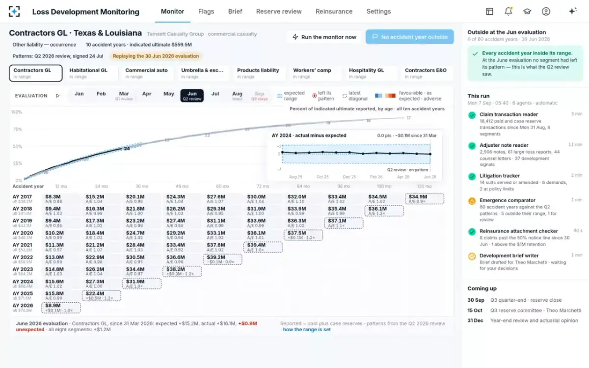
The same replay idea on a live book: step back to the evaluation the last review saw
What the replay cannot tell you
A replay on public annual data is a lower bound on a monitor's value and an imperfect one. The data is annual, so the first evaluation after the review comes twelve months later; a monthly monitor sees the same break up to eleven months sooner, which this data cannot show. The selection is mechanical, so the expected development is a chain ladder pattern, not what a reserving actuary would have chosen. The data is net of reinsurance, so program changes move triangles without any change in claims. The outcome is incurred at ten years including the insurer's own IBNR, a proxy for the ultimate, not the ultimate. And the CAS kept only insurers with complete data in every later statement, so insurers that failed or merged are missing, the ones whose reserves most needed watching.
Nor can the data explain anything. Schedule P carries no claim notes, so the replay can count flags but not say whether the move came from expert reports, suits or a data error. On a real book, the explanation is the larger part of a flag's value: it decides whether the actuary marks it watched, explained or for the reserve review.
How to replay a monitor on your own closed years
Run the same test on your own data, monthly instead of annually, before trusting any monitor's flags. Take the patterns from a review at least three years old, roll the monitor forward month by month on the transactions that followed, and score each flag against how its accident year actually developed. Count the flags that preceded adverse development, the ones that did not, and the adverse years nothing flagged. Then repeat with the range at 70% and 90% of past variation and with a higher dollar threshold, and choose settings with the false-alarm rate your team can live with; the settings and what each changes are set out in the eight settings that decide a flag.
A useful second step is the explanation test. For a sample of the flags that preceded adverse development, read the claims behind the move and ask whether the cause was in the claim notes at the time of the flag. Where it was, the flag would have arrived with its story; where it was not, the monitor bought time but not understanding. The arithmetic behind each flag, expected, actual, range and A/E, is worked through in actual vs expected, cell by cell.
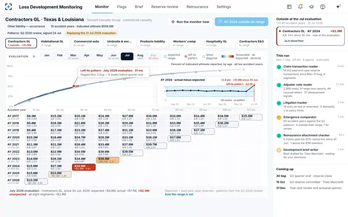
The month the curve left its range, replayed on the sample book
What this means when choosing a reserve monitor
Ask any monitor's supplier the questions this replay answers, on your data: how often did a flag precede adverse development, how often was it a false alarm, how many adverse years did it miss, and how much earlier than the quarterly diagonal did it speak. A supplier who cannot run that test cannot tell you what its flags mean. Loss Development Monitoring's replay scrubber runs it on the solution's own history, month by month, from the signed patterns of a past review; the CAS data is how to check the idea before your own data is connected. Where a monitor sits beside reserving software and stochastic models is compared in actuarial reserving software vs a monitor.
The regulators' own early-warning tools work the same way at a coarser grain. The NAIC's IRIS ratios test one-year and two-year reserve development against surplus, and its manual sends analysts who find reserves that look deficient to Schedule P, Part 2, to work out which lines and which accident years caused it (NAIC IRIS Ratios Manual). A monitor asks the same question inside the company, every month, before the annual statement asks it.
Questions people ask
Is the CAS Schedule P data free?
Yes. The six files for each data set are posted on the CAS research pages and can be downloaded without membership. Each row is one insurer, accident year and development lag, with incurred, paid, bulk and IBNR losses and earned premium.
What years does the CAS loss reserving database cover?
The original set covers accident years 1988 to 1997 and was posted in 2011; a second set covers accident years 1998 to 2007 and is marked as updated in December 2025. Each has ten years of development for every accident year, including the lower triangle.
Why do researchers use Schedule P data for reserving studies?
Because it is the only consistent, public, insurer-level source of loss triangles for US property and casualty business, and the CAS version adds the outcomes. That lets a method be tested on development it never saw, which is what Meyers and Shi did for stochastic models.
What does Schedule P Part 2 show?
Part 2 shows incurred net losses and defense and cost containment expense by accident year at successive year-ends, which is the incurred development triangle. The NAIC's IRIS manual points analysts to Schedule P, Part 2 to find a reserve deficiency by line of business and accident year.
Does a flag in the first year mean the reserve is deficient?
No. In our replay, about half of first-year flags were followed by adverse development and half were not. Two consecutive years outside the range was a stronger signal, followed by adverse development in about four cases in five.
Can the CAS data be used to choose monitoring thresholds?
It can show the trade-off. In our replay on the 1997 set, widening the range from 70% to 90% of past variation cut first-year flags from 323 to 219 and the share of adverse years caught from 37.2% to 26.1%; raising the floor from 0% to 3% of the ultimate cut flags from 308 to 194 and lifted the share followed by adverse development from 44.2% to 57.7%. The final settings should be tested on the insurer's own monthly data.