The burning cost method in reinsurance estimates the expected cost of a treaty layer from the cedant's own loss history: each historical loss is trended to the treaty period, the part that falls in the layer is summed by year, those sums are developed to ultimate, and the total is divided by the subject premium brought to the treaty period's rate level. The result is a loss cost, a percentage of subject premium, which is then loaded for commission, brokerage, expenses and profit to become a rate. Each step is a choice: the trend rate, how policy limits are treated, which development factors, which rate changes. That is where a cedant's burning cost and a reinsurer's part company. Botminds' Treaty Underwriting Workbench rebuilds those inputs from the cedant's own data, with each choice set by the reinsurer and each figure cited.
The worked figures below are the Casualty Actuarial Society's own, from David Clark's study note on reinsurance pricing, so every number can be checked against the source. Examples from the solution use its fictional sample season.
The burning cost formula: four inputs, each a place where two pricers can differ
Trended losses
loss × (1 + trend)^years
Each historical loss, including those just below the attachment, brought to the treaty period's cost level.
Trend source: the pricer's choice
In the layer
min(max(loss − retention, 0), limit)
The part of each trended loss between the attachment and the top of the layer, summed by year.
Policy limits and ALAE treatment
Developed
layer losses × LDF
Each year's layer total taken to ultimate with excess development factors.
Development pattern
On-level premium
premium × rate and exposure factors
The denominator, at the rate level and exposure inflation of the treaty period.
Rate history: filed or achieved
What is burning cost in reinsurance? The raw ratio and the projected one
Burning cost means two things, and the difference matters. Clark's study note for the Casualty Actuarial Society explains: "Experience rating is sometimes referred to as a "burn cost" model though that phrase more commonly denotes just the unadjusted experience and not the projected cost" (Clark, Basics of Reinsurance Pricing). The raw burning cost is past losses in the layer, as they stand today, over past premium. The projected burning cost is what a pricer uses: losses and premium both restated to the treaty period.
The idea behind both is the same: "the historical experience, adjusted properly, is the best predictor of future expectations." The words that carry the weight are "adjusted properly". A raw burning cost from a ten-year history uses losses at prices up to ten years old, premium at rates that have since changed, and young years whose claims have not finished developing. Every one of those biases runs the same way in a period of rising claim costs: the raw ratio understates the future cost.
How do you calculate burning cost? The CAS example, year by year
Clark's worked example prices a property per-risk excess treaty of $400,000 excess of $100,000, effective 1 January 1997, from fourteen losses between 1988 and 1995. Each loss is trended at 4% a year from its accident date to the treaty period, the part above $100,000 and up to $500,000 goes into the layer, the layer losses are summed by accident year, developed, and divided by on-level subject premium.
Burning cost, worked: eight accident years to a 12.4% loss cost
| Accident year | On-level subject premium | Trended losses in layer | Development factor | Trended ultimate in layer | Loss cost |
|---|---|---|---|---|---|
| 1988 | 1,422,554 | 639,975 | 1.000 | 639,975 | 45.0% |
| 1989 | 1,823,103 | 119,009 | 1.000 | 119,009 | 6.5% |
| 1990 | 2,054,034 | 51,661 | 1.000 | 51,661 | 2.5% |
| 1991 | 2,147,147 | 109,505 | 1.000 | 109,505 | 5.1% |
| 1992 | 2,151,541 | 323,357 | 1.010 | 326,591 | 15.2% |
| 1993 | 2,159,198 | 214,331 | 1.050 | 225,048 | 10.4% |
| 1994 | 2,167,158 | 0 | 1.150 | 0 | 0.0% |
| 1995 | 2,187,654 | 400,000 | 1.300 | 520,000 | 23.8% |
| Total | 16,112,389 | 1,857,838 | 1,991,789 | 12.4% |
Three things stand out. First, the answer is volatile by year: from 0.0% to 45.0%, because a per-risk layer sees a handful of losses. Clark's note expects the yearly loss costs to scatter around their average, and treats a steady rise or fall across the years as a sign that the trend or development assumptions need another look. Second, two losses reach the full $400,000 limit, so two events carry almost half the total. Third, the youngest year carries the biggest development factor: 1995's single limit loss of $400,000 becomes $520,000 at a factor of 1.300, adding $120,000, six percent of the total, on a judgment about how that year will finish.
How are losses trended for reinsurance pricing? Why a layer feels inflation more
Losses are trended by applying an annual inflation rate from each loss's accident date to the average date of the treaty period; the question is which rate. Clark lists the cedant's own figures among the options: "Various sources are available for this adjustment, including the amounts used in the ceding company's own rate filings." For casualty he adds that the selection "is difficult", that an unlimited trend derived from large losses only is what theory wants, and that "In the final analysis, the actuary must make a selection of loss inflation rates by year."
Trend matters more for a layer than for the losses beneath it. Patrik's chapter in the CAS textbook explains why trending may not be skipped for excess cover: "a constant inflation rate increases the aggregate loss above any attachment point faster than the aggregate loss below, because claims grow into the excess layer, while their value below is stopped at the attachment point" (Patrik, Foundations of Casualty Actuarial Science, ch. 7). Clark's own data shows it.
Trend a loss by a third and its share of the layer more than triples
The bars also show the other edge of a layer. Two of Clark's losses, $821,499 and $771,249 before trend, were above the layer's top before any adjustment, so trend adds nothing to them; the layer is capped. A layer is leveraged at the bottom and capped at the top, and which effect wins depends on where its losses sit. That is why Patrik wants detail on every claim near the layer: "We usually receive information on all claims greater than one-half the proposed attachment point, but, the more data, the better." A listing that starts at the attachment point misses the claims that trend will push into it.
Development: the factor that decides the latest years
Development takes each year's layer losses from what is known today to what they will finally cost, and on a layer the younger years can be mostly development. In Clark's property example the factors are modest, 1.010 to 1.300, because property claims settle fast. On casualty layers they are not: Clark notes that the factors needed are "very large", that the excess patterns should come from the cedant's own data where possible, and that a benchmark should be used where it is not.
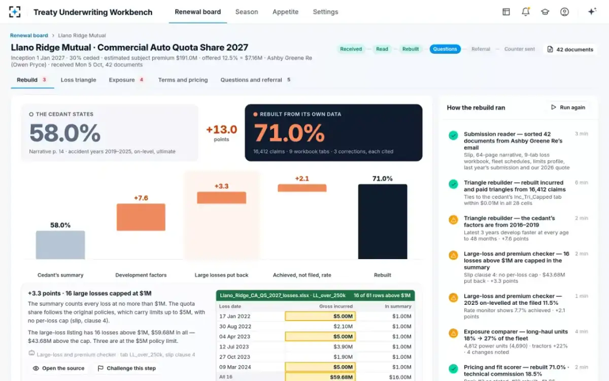
The sample program in the Treaty Underwriting Workbench shows the scale on a casualty book. Llano Ridge Mutual's commercial auto triangle, rebuilt from 16,412 claims, takes a twelve-month year to ultimate at 2.51 on its own latest three years; the cedant's summary used factors selected from 2016–2019 that give 1.78. On the same premium that one choice moved the loss ratio by 7.6 points. How to test a rebuilt triangle before trusting it is set out in replaying a loss development triangle.
What is on-level premium? The denominator moves too
On-level premium is historical subject premium restated at the rate level, and exposure level, expected in the treaty period; without it, a year written at old, lower rates looks worse than it would at today's rates. Clark's proportional example uses on-level factors from 0.992 to 1.096 for six years of earned premium, from rate changes of +2%, +10%, −4% and a pending +10%, by "a standard parallelogram method", and trends premium for 3% annual property value inflation as well.
Clark flags the judgment in the last rate change: the impact of rate changes during the treaty period "must also be included. This is an area requiring some judgment, as these percents may not actually have been filed or approved at the time the treaty is being evaluated." The same judgment applies backwards. A rate the cedant filed is not necessarily the rate it achieved on renewals, and on-levelling with the filed rate inflates the denominator. On the sample program the cedant on-levelled 2025 with its filed 11.5%; its own rate monitor showed 7.7% achieved, and the difference was worth 2.1 points of loss ratio.
Policy limits and large losses: history restated to today's terms
A burning cost must count each historical loss as it would fall under the treaty being priced, and for casualty the policy limits make that hard. Clark calls capping trended losses at applicable policy limits "another problem for which there is no generally accepted solution". Applying the historical limit to a trended loss ignores the fact that insureds buy higher limits over time; trending without any cap assumes limits "drift" upwards exactly with inflation, in which case the premium must also be restated to what the higher limits would have cost.
The cedant's summary can make this worse by capping losses for its own reasons. In the sample, Llano Ridge's summary counted every loss at no more than $1 million, though the quota share follows original policies with limits up to $5 million and has no per-loss cap (slip, clause 4). The large-loss listing held sixteen losses above $1 million, $59.68 million in all, $43.68 million above the cap; three were at the $5 million policy limit. Putting them back to the treaty's own terms added 3.3 points. Clark's proportional method sets catastrophe and shock losses aside so they do not distort the base, then loads the expected loss ratio for catastrophes; leaving large losses out with nothing added back is what makes a summary flattering.
A step, with its evidence: sixteen large losses put back to the treaty's terms
Burning cost vs exposure rating: history against today's book
Burning cost prices from what the cedant has lost; exposure rating prices from what it now writes. Clark puts the case for the second plainly: "the current risk profile is modeled, not what was written years earlier." It uses the cedant's limits profile and a severity curve, so it sees a layer even where the history shows no losses in it. Each method covers the other's weakness, and the pricer weighs them.
Burning cost and exposure rating answer different questions; a pricer needs both
Burning cost (experience rating): The cedant's own historical losses and premium.
Exposure rating: The cedant's current limits profile and premium, and a severity curve built from industry statistics.
Burning cost (experience rating): Reflects this cedant's actual claims, underwriting and claims handling.
Exposure rating: Reflects the book as written today, including limits and classes the history never tested.
Burning cost (experience rating): Few losses in a layer make it volatile; changes in the book since the history make it stale.
Exposure rating: The curve is not this cedant's; the result moves in proportion to the assumed loss ratio.
Burning cost (experience rating): No historical loss reached the top of the layer: the "free cover" problem.
Exposure rating: The limits profile is wrong, for example by policy rather than by location.
Burning cost (experience rating): Should rest on the number of claims expected in the period, not the number observed.
Exposure rating: Clark notes that experience rating often gets significant weight simply because exposure rating has too many limitations.
The "free cover" row is the burning cost's best-known blind spot. Clark describes an experience rating "in which no losses trend into the highest portion of the layer being priced": price a $750,000 excess of $250,000 layer and a $250,000 excess of $250,000 layer from a history whose largest trended loss is $500,000, and both get the same loss cost, so the upper $500,000 is priced at nothing. His suggested fix is to use the experience rate for the lower part of the layer and the exposure curve's relativities for the rest. On credibility he warns against rewarding bad luck: credibility should rest on the number of claims expected, because if it rests on the number observed, "more credibility will be assigned to experience rating projections that are fortuitously worse than average."
Where a cedant's burning cost and a reinsurer's part company
A cedant and a reinsurer can run the same method on the same losses and reach different numbers without either making an arithmetic error. The differences sit in six choices, and a broker will only accept the reinsurer's number if each choice is shown.
Six choices that separate the cedant's burning cost from the reinsurer's
- Trend source and rate
The cedant's filed trend, a ground-up index, or an excess trend from large losses only.
- Development factors
Which years they are selected from, volume-weighted or averaged, and which tail.
- Policy limits on trended losses
Historical limits, limits that drift with inflation, or the limits profile written today.
- Large-loss treatment
Capped as shock losses and loaded back separately, or left to the treaty's own terms.
- Premium on-level
Filed rate changes or achieved ones from the cedant's rate monitor.
- ALAE and inuring cover
Pro rata with loss or added to it; losses net of any reinsurance that inures to this treaty.
In the sample, three of those six choices explained the whole gap between Llano Ridge's 58.0% and the rebuilt 71.0%: development (+7.6), large losses (+3.3) and the on-level rate (+2.1). Each is a step on a bridge, cited to the tab, cell or page it came from, which is the form a broker can argue with. The bridge itself, and why the cedant's number and the reinsurer's differ, is the subject of the as if loss ratio.
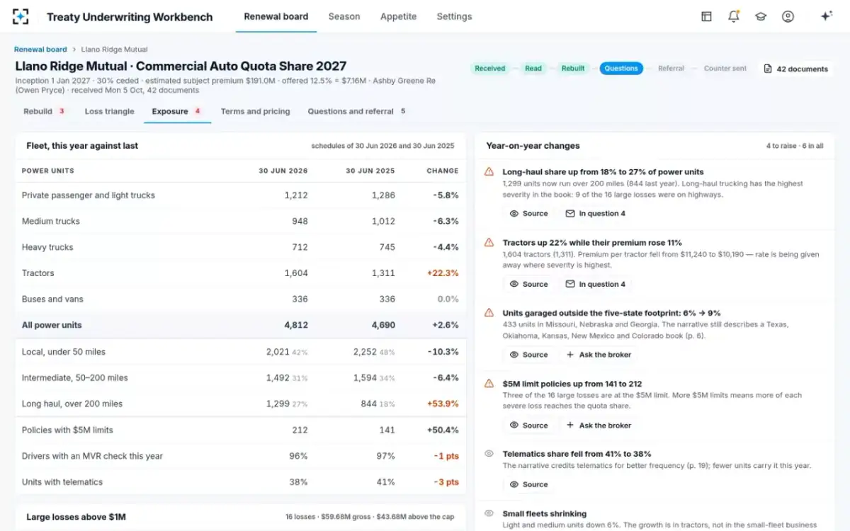
Exposure year on year: the history a burning cost reads may not be the book being reinsured
To see a cedant's losses rebuilt to your own trend, development and on-level rules, start from the Treaty Underwriting Workbench.
Questions people ask
What is the difference between burning cost and loss ratio?
A loss ratio usually compares a book's total losses with its premium; a burning cost compares only the losses that fall in a reinsurance layer with the subject premium. In Clark's CAS example the treaty layer's burning cost is 12.4% of subject premium, a number that would mean nothing as a loss ratio for the cedant's whole book.
How many years of losses should a burning cost use?
Enough to be credible, recent enough to be relevant. Clark's study note suggests about ten years for a per-risk excess layer and says the number relied on should balance credibility against responsiveness; long-tail casualty layers often need more years and lean harder on development and exposure rating.
What is free cover in reinsurance pricing?
It is the part of a layer that a burning cost prices at nothing because no historical loss, even after trend, reached it. Clark's example: if the largest trended loss is $500,000 from the ground up, a $750,000 excess of $250,000 layer gets the same loss cost as $250,000 excess of $250,000, so the top $500,000 is implicitly free.
Can the burning cost method price a quota share?
The same steps apply, but a quota share is usually priced as an expected loss ratio for the whole book, then judged through the ceding commission it can afford, often on a sliding scale. Clark's proportional example projects six years to a 54.6% non-catastrophe loss ratio, loads 10% for catastrophes and tests a suggested 30% commission, which gives a 102% combined ratio.
How do you turn a burning cost into a reinsurance rate?
Load it for what the premium must also pay: ceding commission if any, brokerage, the reinsurer's expenses and its target return. Patrik's CAS chapter writes the rate as the expected loss cost divided by the share of premium left after each of those, so the loss cost is always smaller than the rate it supports.