A performance attribution analysis example is easiest to follow on a real-shaped report: a global equity strategy returned 1.84% in a quarter against 3.26% for its index, and the attribution report splits that 142 basis point (bp) gap into four effects, allocation −39bp, selection −94bp, interaction −1bp and currency −8bp, sector by sector. Every cell is a product of a weight difference and a return difference, every row adds across, and every column adds down to the active return. The hard part of performance attribution analysis is rarely the arithmetic; it is knowing which three cells matter and finding the decision behind each. Botminds' Performance Attribution Analysis reads the official report, ties each sentence of an answer to the cells it uses, and checks that they add up before a performance analyst signs.
The report on this page is sample data from the solution: Global Equity, a fictional strategy of the fictional Quillfield Capital, third quarter of 2026, measured against the equally fictional Norvale Global All Cap Index. The figures are the solution's own, and every cell can be recomputed from the weights and returns shown.
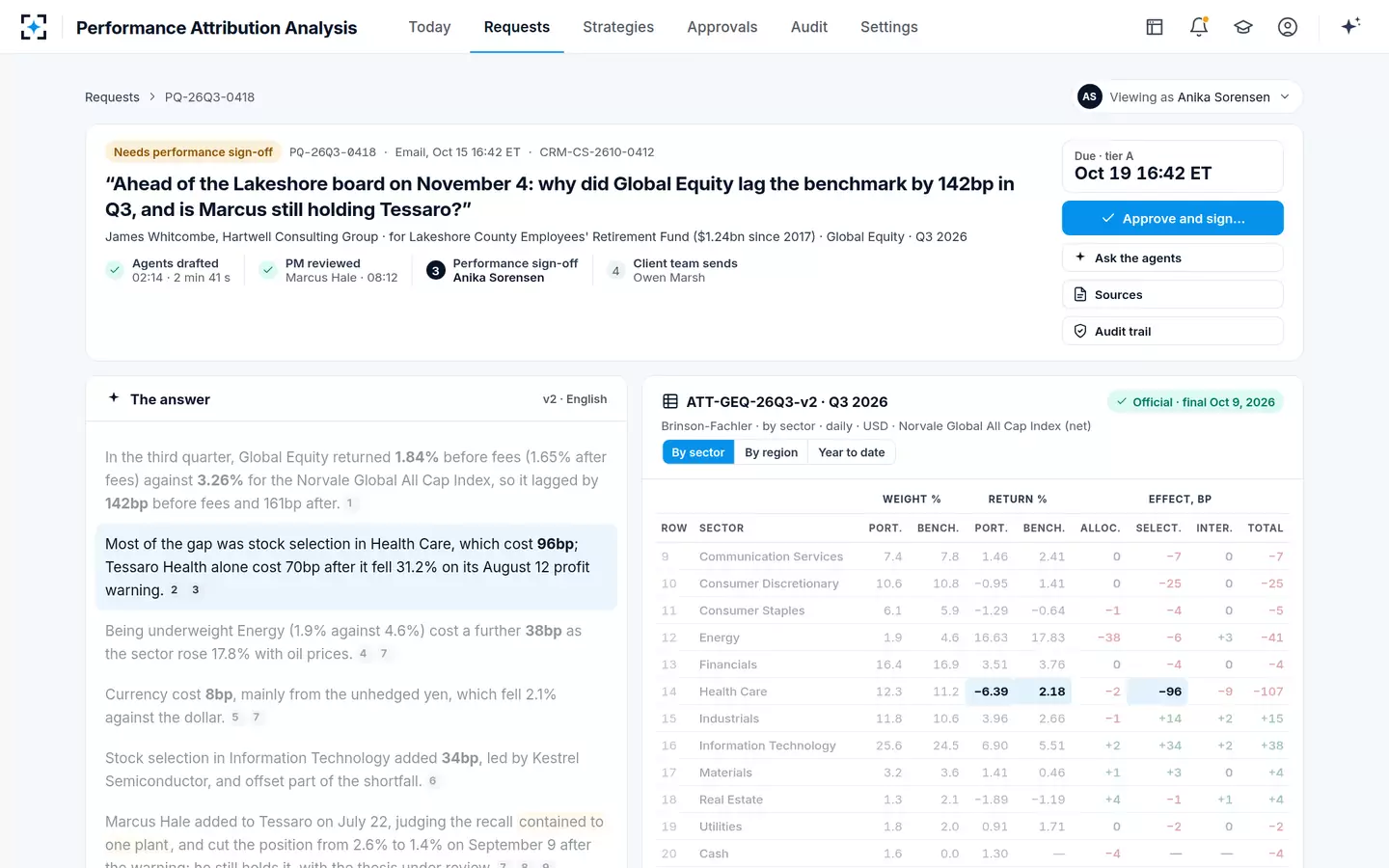
The whole Global Equity report: eleven sectors and cash, four numbers each
Communication Services
Weight P / B, %7.4 / 7.8
Return P / B, %1.46 / 2.41
Alloc.0
Select.−7
Inter.0
Total−7
Consumer Discretionary
Weight P / B, %10.6 / 10.8
Return P / B, %−0.95 / 1.41
Alloc.0
Select.−25
Inter.0
Total−25
Consumer Staples
Weight P / B, %6.1 / 5.9
Return P / B, %−1.29 / −0.64
Alloc.−1
Select.−4
Inter.0
Total−5
Energy
Weight P / B, %1.9 / 4.6
Return P / B, %16.63 / 17.83
Alloc.−381
Select.−6
Inter.+3
Total−41
Financials
Weight P / B, %16.4 / 16.9
Return P / B, %3.51 / 3.76
Alloc.0
Select.−4
Inter.0
Total−4
Health Care
Weight P / B, %12.3 / 11.2
Return P / B, %−6.39 / 2.18
Alloc.−2
Select.−962
Inter.−93
Total−107
Industrials
Weight P / B, %11.8 / 10.6
Return P / B, %3.96 / 2.66
Alloc.−1
Select.+14
Inter.+2
Total+15
Information Technology
Weight P / B, %25.6 / 24.5
Return P / B, %6.90 / 5.51
Alloc.+2
Select.+34
Inter.+2
Total+38
Materials
Weight P / B, %3.2 / 3.6
Return P / B, %1.41 / 0.46
Alloc.+1
Select.+3
Inter.0
Total+4
Real Estate
Weight P / B, %1.3 / 2.1
Return P / B, %−1.89 / −1.19
Alloc.+4
Select.−1
Inter.+1
Total+4
Utilities
Weight P / B, %1.8 / 2.0
Return P / B, %0.91 / 1.71
Alloc.0
Select.−2
Inter.0
Total−2
Cash
Weight P / B, %1.6 / 0.0
Return P / B, %1.30 / —
Alloc.−44
Select.—
Inter.—
Total−4
Effects, local currency
Weight P / B, %100 / 100
Return P / B, %2.33 / 3.66
Alloc.−39
Select.−94
Inter.−1
Total−134
What a performance attribution report shows, in one line per sector
Each row of an attribution report answers one question about one slice of the portfolio: did the manager hold more or less of it than the index, and did the holdings inside it beat the index's holdings? The first two column pairs are the evidence, the portfolio's and the benchmark's weight and return in that sector. The effect columns are the verdict, in basis points of the whole portfolio, not of the sector.
That last point is where most first readings go wrong. Health Care's portfolio return was −6.39% against 2.18% for the index's Health Care stocks, a gap of 8.57 percentage points. The report does not show 857bp. It shows −96bp of selection, because the sector was about a ninth of the index and the effect is scaled to the whole portfolio. A reader who sees a sector with a dreadful return and a modest effect is looking at a small sector; a reader who sees a mediocre return and a large effect is looking at a big one.
The method is the one Gary Brinson and Nimrod Fachler published for non-US equity portfolios in 1985 (Journal of Portfolio Management 11(3)), and on the decomposition Brinson, Hood and Beebower set out a year later (Financial Analysts Journal 42(4)). Versions of this grid differ in two places, how allocation is measured and where interaction goes, and both are covered below.
The top line: 142bp before fees, 161bp after, and a currency step
Start where a consultant starts: the strategy returned 1.84% before fees and 1.65% after, against 3.26% for the index, so it lagged by 142bp before fees and 161bp after. The 19bp difference is fees and expenses, not a market effect, and it never appears in this grid: the report is calculated before fees, which is why any answer quoting it has to say so and show the after-fee figure beside it.
The grid's own returns do not match the top line, and that is the second thing to check. Multiply each sector's weight by its return and add: the portfolio comes to 2.33% and the index to 3.66%. Those are local-currency returns. In US dollars the two were 1.84% and 3.26%, so translation took about 49bp from the portfolio and 40bp from the index, roughly 9bp more from the fund. The report's currency effect is the same gap measured against its linked effects: −142bp in dollars less −134bp in local currency, or −8bp. It is the cost of the fund's currency exposures, mainly unhedged yen, relative to the index's own.
Four terms add to the active return; each is a weight gap times a return gap
Allocation
(wP − wB) × (rB,sector − RB)
Over- or underweighting a sector, scored by how that sector did against the whole index.
Energy: −2.7% × 14.17% = −38bp
Selection
wB × (rP,sector − rB,sector)
Picking better or worse stocks than the index within a sector, at the index’s weight.
Health Care: 11.2% × −8.57% = −96bp
Interaction
(wP − wB) × (rP,sector − rB,sector)
The joint effect of holding a different weight of a sector whose stocks also did differently.
Health Care: 1.1% × −8.57% = −9bp
Currency
USD active − local active
What translating local returns into the reporting currency did to the gap.
−142bp − (−134bp) = −8bp
How is the allocation effect calculated? The Energy cell, worked
The allocation effect is the weight difference in a sector multiplied by how much that sector beat or trailed the whole benchmark. In this report Energy carried 1.9% of the portfolio against 4.6% of the index, an underweight of 2.7 percentage points. Energy stocks in the index returned 17.83% in local currency, 14.17 points more than the index's 3.66%. Allocation is −2.7% × 14.17%, or −0.38%: −38bp, cell (1) in the grid.
The intuition, in the words of a peer-reviewed description of the model, is that "a portfolio would produce different returns with different allocation schemes" while keeping "the same stock selection and thus the same return" in each category (Lu and Kane, The R Journal, 2013). Allocation asks what the weights alone did, holding every sector at the index's own return. The answer here: being light in the best-performing sector of the quarter cost 38bp, more than a quarter of the shortfall.
Notice what the formula does not use: the portfolio's own Energy return. The fund's Energy stocks rose 16.63%, a strong quarter by any measure, and it still lost 38bp of allocation. A sentence like "Energy hurt us" is therefore wrong, and "not owning enough Energy hurt us" is right. The distinction matters because consultants read the sentence, not the cell.
How is the selection effect calculated? The Health Care cell, worked
The selection effect is the benchmark's weight in a sector multiplied by the gap between the portfolio's and the index's return inside it. Health Care was 11.2% of the index; the portfolio's Health Care stocks returned −6.39% against 2.18% for the index's, a gap of −8.57 points. Selection is 11.2% × −8.57%, or −0.96%: −96bp, cell (2), the largest number in the report.
Using the benchmark weight is a choice, and it is the reason a separate interaction column exists. It scores stock picking as if the manager had held Health Care at the index's weight, so the selection number is not inflated or shrunk by the manager's own allocation bet. In the sample, one holding, Tessaro Health, accounts for about 70bp of the 96: its shares fell 24.1% on the day of an August profit warning and 31.2% over the quarter.
Three cells explain the quarter: Health Care selection, Energy allocation, IT selection
The interaction column, and why it is usually small
Interaction is what is left when allocation and selection have each been scored on their own: the weight difference multiplied by the return difference. Health Care was overweight by 1.1 points and its stocks lagged by 8.57, so interaction is 1.1% × −8.57%, or −9bp, cell (3). The manager held slightly more of a sector in which his stocks did badly, and the two decisions compounded each other.
For most rows interaction is close to zero, because either the weight gap or the return gap is small. In this report it sums to −1bp across the portfolio: Health Care's −9 offset by small positives in Energy, Industrials and IT. Some firms fold it into selection and never show it; this report shows it, and who owns the interaction effect takes the question further, including what a commentary must not say about it.
Brinson-Fachler vs Brinson-Beebower: same total, different Energy cell
The two models give the same total allocation and different sector cells. Brinson, Hood and Beebower score allocation as the weight difference times the sector's own benchmark return; Brinson and Fachler subtract the whole benchmark's return first. Because the weight differences across all sectors and cash add to zero, the subtraction cancels in the total, but it moves money between rows.
The same weights, two allocation formulas: totals agree, sectors do not
| Sector | Weight gap | Brinson-Beebower: gap × sector return | Brinson-Fachler: gap × (sector − index) |
|---|---|---|---|
| Energy | −2.7% | −48bp | −38bp |
| Health Care | +1.1% | +2bp | −2bp |
| Information Technology | +1.1% | +6bp | +2bp |
| Cash | +1.6% | +2bp | −4bp |
| All sectors and cash | 0.0% | ≈ −37bp | ≈ −37bp |
The Health Care line is the reason most firms use Brinson-Fachler. Under Brinson-Beebower, overweighting Health Care earned +2bp simply because Health Care stocks went up, even though they went up less than the index. Under Brinson-Fachler the same overweight cost 2bp, because money placed in Health Care would have done better in the index as a whole. Cash shows the same flip: positive under one formula for earning 1.30%, negative under the other for earning less than the 3.66% the index made.
What does a negative allocation effect mean?
A negative allocation effect means the manager was overweight a sector that trailed the benchmark or underweight one that beat it. Under Brinson-Fachler the sign comes from two signs multiplied: the weight gap and the sector's return relative to the index. Overweight and outperforming, or underweight and underperforming, is positive; the mixed cases are negative.
The sample report has both negative cases. Energy is underweight and outperforming: −38bp. Cash is overweight and underperforming: −4bp, the familiar cash drag of a rising market. Real Estate is the mirror image of Energy, underweight a sector that fell 1.19% while the index rose, and it earned +4bp. None of these says anything about the stocks held; that is selection's job. And a negative allocation in a sector the mandate excludes, such as Energy in a fossil-fuel-free version of the same strategy, is a cost of the client's restriction rather than a decision anyone made in the quarter.
The same grid in Performance Attribution Analysis, with the sentence that relies on row 14 lit
How to do performance attribution analysis in Excel, column by column
To do performance attribution analysis in Excel, lay out one row per sector with four inputs, compute the two total returns, then add one column per effect. The layout below reproduces the sample report's cells to within a basis point. It is a single-period calculation: a spreadsheet that does this for each day or month and then compounds the results is a much larger job, which is where most firms stop using spreadsheets.
A single-period Brinson-Fachler sheet: four inputs, two totals, four effects
| Column | Holds | Formula in row 2 (rows 2–13 are sectors) | Energy result |
|---|---|---|---|
| B, C | Portfolio and benchmark weight | inputs, each column summing to 100% | 1.9%, 4.6% |
| D, E | Portfolio and benchmark sector return | inputs, local currency | 16.63%, 17.83% |
| Totals | Whole-portfolio returns | =SUMPRODUCT(B2:B13,D2:D13) and =SUMPRODUCT(C2:C13,E2:E13) in D14, E14 | 2.33%, 3.66% |
| F | Allocation | =(B2-C2)*(E2-$E$14) | −0.38% |
| G | Selection | =C2*(D2-E2) | −0.06% |
| H | Interaction | =(B2-C2)*(D2-E2) | +0.03% |
| I | Row total | =F2+G2+H2 | −0.41% |
| Check | Sum of I equals D14 − E14 | =ROUND(SUM(I2:I13)-(D14-E14),6)=0 | TRUE |
Two details decide whether the sheet ties. The total returns must be computed from the same weights and returns as the effects, not typed in from the factsheet, or currency and fees will leak into the check. And a selection column that uses the portfolio weight instead of the benchmark weight, =B2*(D2-E2), silently folds interaction into selection; the sheet will still add up, which is why the check proves arithmetic, not method.
Proving the report adds up before anyone reads it
An attribution report should be tested before it is explained, because a wrong number explained well is worse than no explanation. The checks are mechanical and quick, and each catches a different failure that would otherwise reach a client.
Five tie-outs a performance attribution report should pass before anyone explains it
- Each row adds across
Allocation + selection + interaction = row total, within rounding. A row that does not add has a formula or a rounding fault.
- Each column adds down
Sector effects sum to the effect totals: −39, −94 and −1 in the sample.
- Effects add to the local active return
2.33% − 3.66% = −134bp. If not, weights or returns are inconsistent with the totals.
- Currency closes the gap to the reported returns
−134bp + −8bp = −142bp, which matches 1.84% − 3.26%. A gap here usually means a currency or a pricing difference.
- The period is final
A report from a preliminary period can change; any explanation of it can change with it.
Most of these checks are also the ones a reviewer applies to a hand-written answer, and doing them once on the report rather than once per answer saves the same work being repeated for every consultant who asks. The difference between holdings-based reports like this one and reports built from transactions, and what the gap between them can hide, is the subject of transaction vs holdings based attribution.
From cells to sentences: what Performance Attribution Analysis writes
A report becomes an answer when three or four cells become three or four sentences, each with its reason. The SEC asks the same of a fund's annual shareholder report: summarize the key factors that affected performance, and, in the form's own instruction, "Do not include a lengthy, generic, or overly broad discussion of the factors that generally affected market performance during the reporting period" (Form N-1A Item 27A(d)(1), Instruction 1, adopted 2022). Consultants ask for the same discipline, more often.
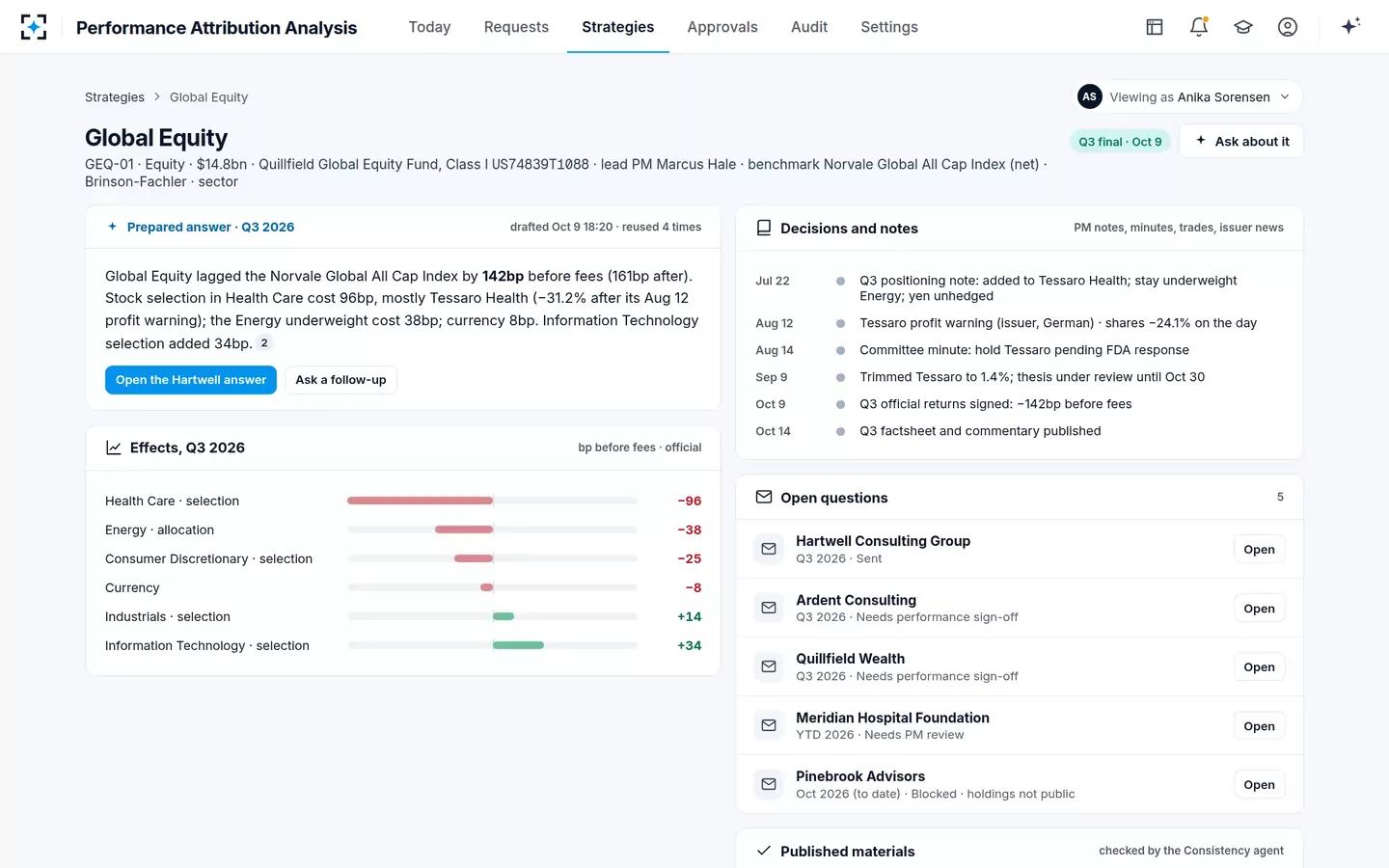
In the sample, the solution's answer has six sentences for 142bp. The first gives the before- and after-fee gap. The second takes cell (2), Health Care selection, and names Tessaro Health. The third takes cell (1), the Energy underweight. The fourth gives currency, the fifth the offset from IT selection, and the sixth quotes the portfolio manager's own note on why he held Tessaro. Consumer Discretionary's −25bp, the interaction column and cash go unnamed: an answer that named every cell would bury the three that matter, and which cells must be named is a firm's own rule, set in the solution as a materiality threshold.
The strategy page: the prepared answer and the effects it rests on
What no report contains is the reason. The −96bp tells a reader where to look, not why the manager held Tessaro or why he cut it in September; that sits in the PM's July note and the trade blotter. The roles that carry an answer from the grid to the consultant are set out in who answers "why did we lag?", and the solution itself, with its checks and sign-off, is at Performance Attribution Analysis.
Questions people ask
What is a simple performance attribution analysis example?
A fund holds 2% of a sector that is 5% of its index, and that sector beats the index by 10 points: under Brinson-Fachler the underweight costs −3% × 10%, or −30bp of allocation. If the fund's own stocks in the sector also trailed the index's by 2 points, selection is 5% × −2%, or −10bp, and interaction is −3% × −2%, or +6bp.
Allocation effect vs selection effect: which matters more?
It depends on the mandate. A sector-neutral manager has allocation close to zero by design, so selection is the whole story; a top-down manager may run large sector bets. In the sample report, selection (−94bp) mattered more than allocation (−39bp), and one holding produced most of the selection loss.
What should a performance attribution report example for a board include?
The before- and after-fee returns of the portfolio and its benchmark, the effect totals, and the two or three largest cells with one sentence each on the decision behind them. A board rarely needs the full grid; it needs to see that the effects add to the gap and that the period is final.
Why does my attribution not add up to the excess return?
Usually because the effects are in local currency and the excess return is in the reporting currency, as in the sample, where −134bp of effects plus −8bp of currency make −142bp. Other causes are fees included in one figure and not the other, a cash row left out, or daily effects summed instead of compounded over the period.
Do I need geometric attribution for a single quarter?
Not usually. Arithmetic Brinson attribution adds exactly for a single period. The difficulty starts when quarters or days are combined, because returns compound and arithmetic effects do not, which is why multi-period reports use a linking method.